What happens to value in sideways markets: Shiller PE and expected returns using Hussman’s method

Robert Shiller’s cyclically adjusted price earnings (CAPE) ratio takes a 10-year inflation-adjusted average of the S&P500’s earnings to arrive at a price/earnings metric smoothed for the business cycle.

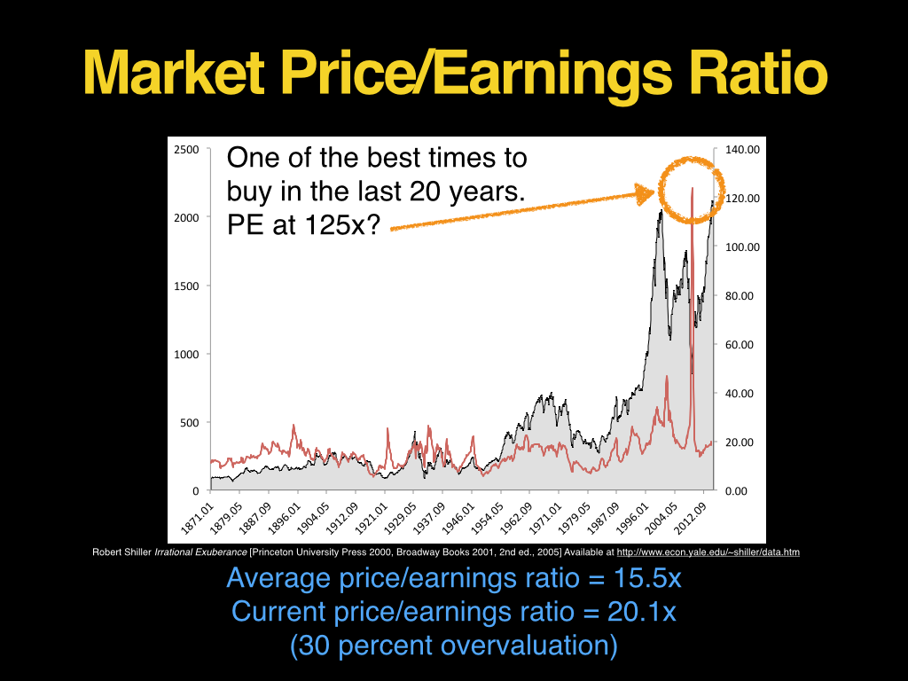
It’s useful because earnings tend to be volatile and mean reverting. For example, the single-year PE metric peaked in 2009 at 125, indicating that the market was expensive, when in reality it was one of the best times to buying stocks in the last 20 years.

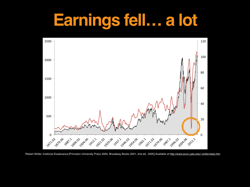
The reason the PE looked so high was because the “E”–earnings–had fallen so far.

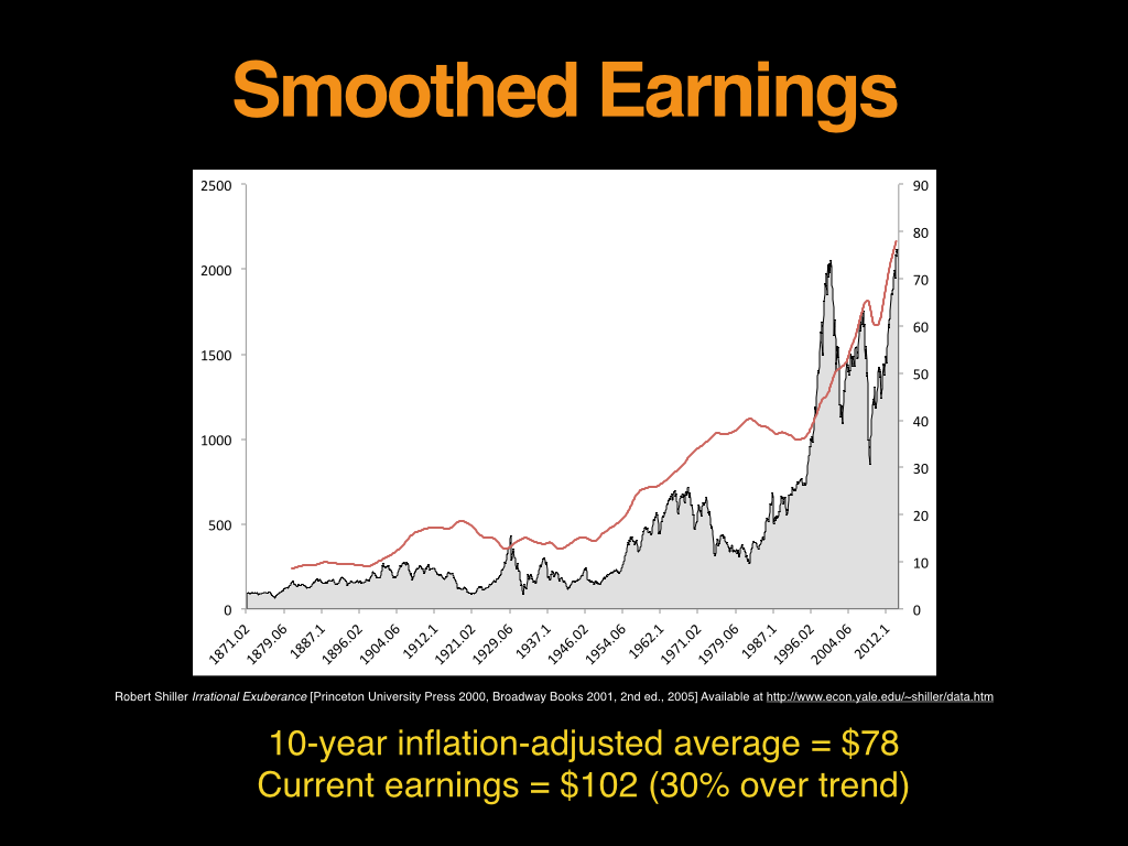
Shiller’s solution is to smooth the earnings by taking the 10-year, inflation adjusted average.

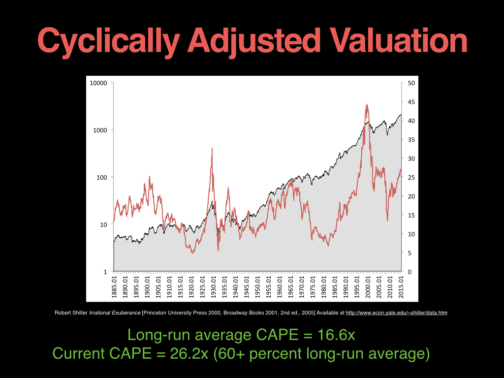
The Shiller CAPE allows us to compare the smoothed earnings to the level of the market and arrive at a cyclically adjusted PE.

The CAPE is currently about 60 percent over its long-run average. Half of the premium comes from earnings 30 percent above trend, and half comes from a single-year multiple 30 percent above its average.

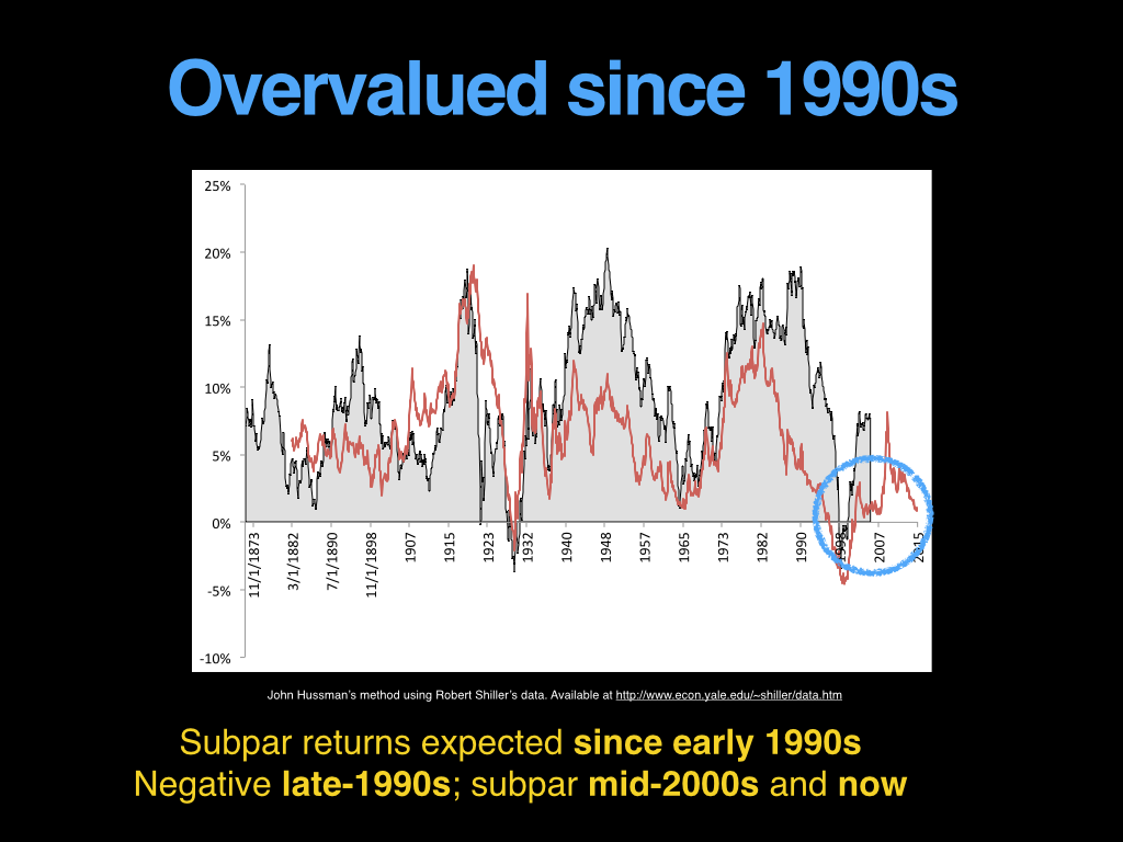
The bulls argue that this premium is justified (or non-existent) because interest rates are low, earnings will stay elevated because US companies earn a greater share of income internationally, and the market has peaked at higher Shiller PEs in the past: 1929 peaked 33x, 2000 peaked at 44x, Japan got to 100x in the 1990s, and China has traded at 100x this year. They also point to the fact that the Shiller PE has indicated the market has been consistently overvalued since the 1990s, only briefly touching the long-run average in the depths of 2009.

John Hussman has a method for calculating 10-year expected returns from Shiller PEs that assumes mean reversion in the PE over the 10 years. The slide below runs the data back to 1871 and compares Hussman’s expected 10-year returns against the returns that actually occur.

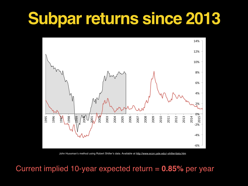
If we zoom in on the area under the blue circle, we can see that Hussman’s method has been predicting below average returns since the mid-1990s, with a deep trough in 1999, and a smaller trough in 2007.

The first trough preceded the 2000 tech bust, and manifest in negative returns for that 10-year period. The second trough preceded the 2007-2009 credit crisis, but has not yet manifest in below average returns (returns are about average for the period), largely because the market has moved back into steep overvaluation. It wouldn’t take much of a move down (as the market has tended to do after below average expected returns emerge) for the actual returns to move down too.

The tool below draws data from Shiller’s site and updates automatically, so bookmark it for future reference.

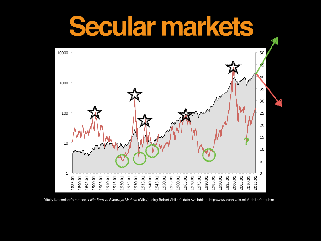
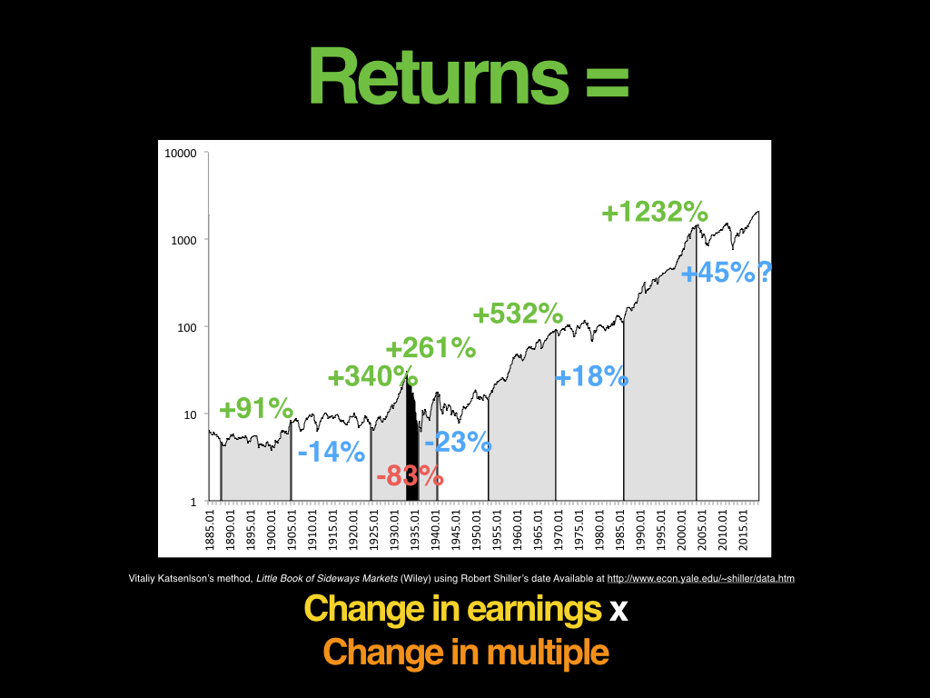
In his Little Book of Sideways Markets, Vitaliy Katsenelson has argued for “secular” markets that emerge as the market moves between distinct Shiller PE peaks and troughs.

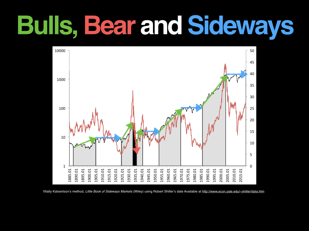
The starred peaks below are the start of infamous crashes–1929, 1966, and 2000–and the circled troughs are the start of blistering bulls–1920, 1950, and 1982 (and maybe 2009 if the bulls are right). Katsrnelson argues that these secular turning markets appear as bull markets, and sideways markets (rather than bear markets–Katsenelson argues that 1929 is a special case because the market fell so far, ~90 percent).

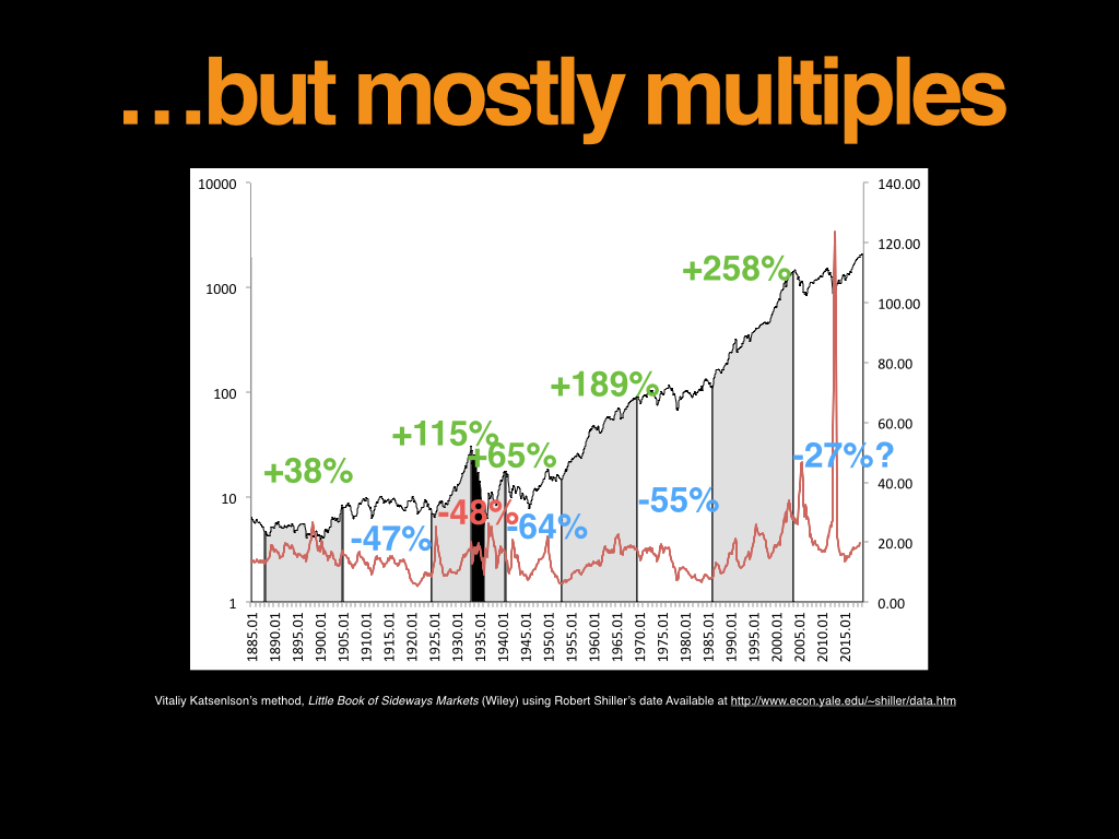
The returns in securlar markets are driven more by changes in the multiple applied to earnings, than earnings themselves, which have been consistently up.

Earnings have grown pretty consistently over the full period.

So changes in the multiple applied to the earnings has been the difference in returns.

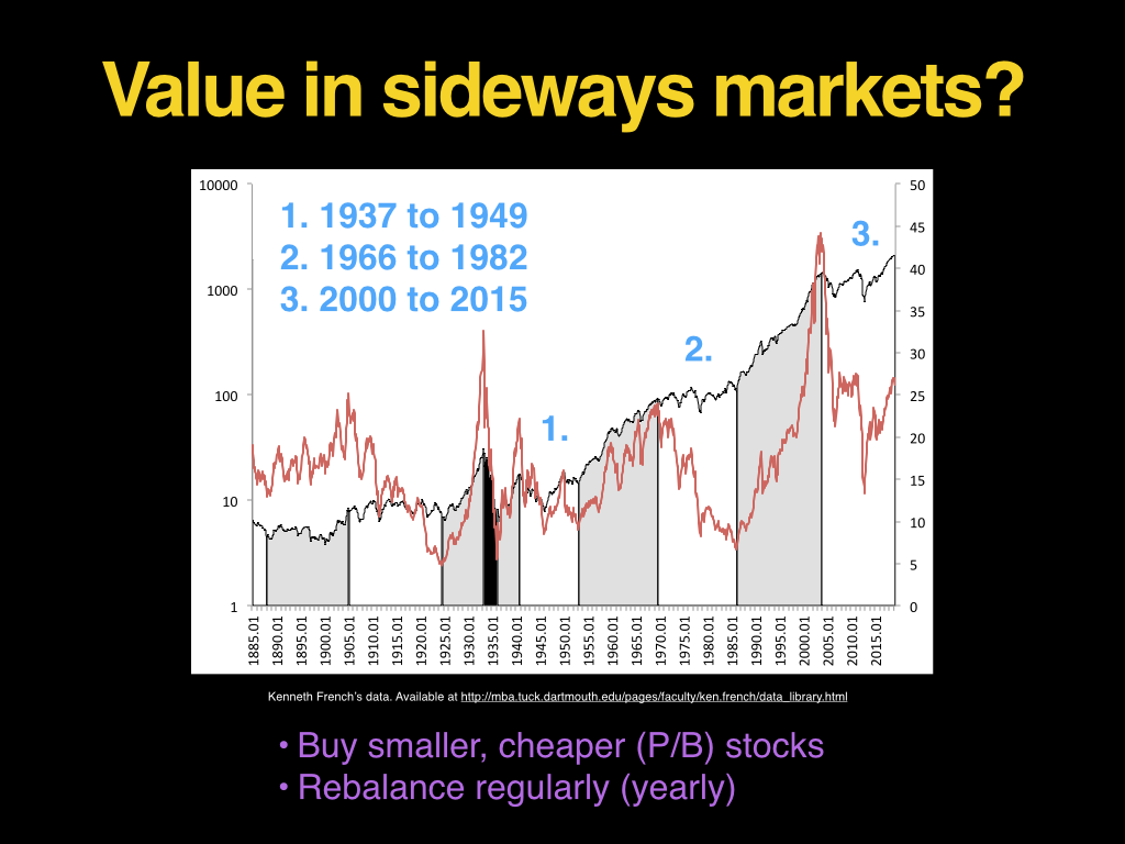
Of course, the level of the market is less interesting to value investors who are (or should be) focussed on the market’s undervalued dreck. Value seems to follow its own idiosyncratic path, correlated to, but distinct from the market itself. The interesting question is, “What happens to value stocks in sideways markets?” The three most recent sideways markets, which followed big bull markets, started in 1937, 1966 and 2000.

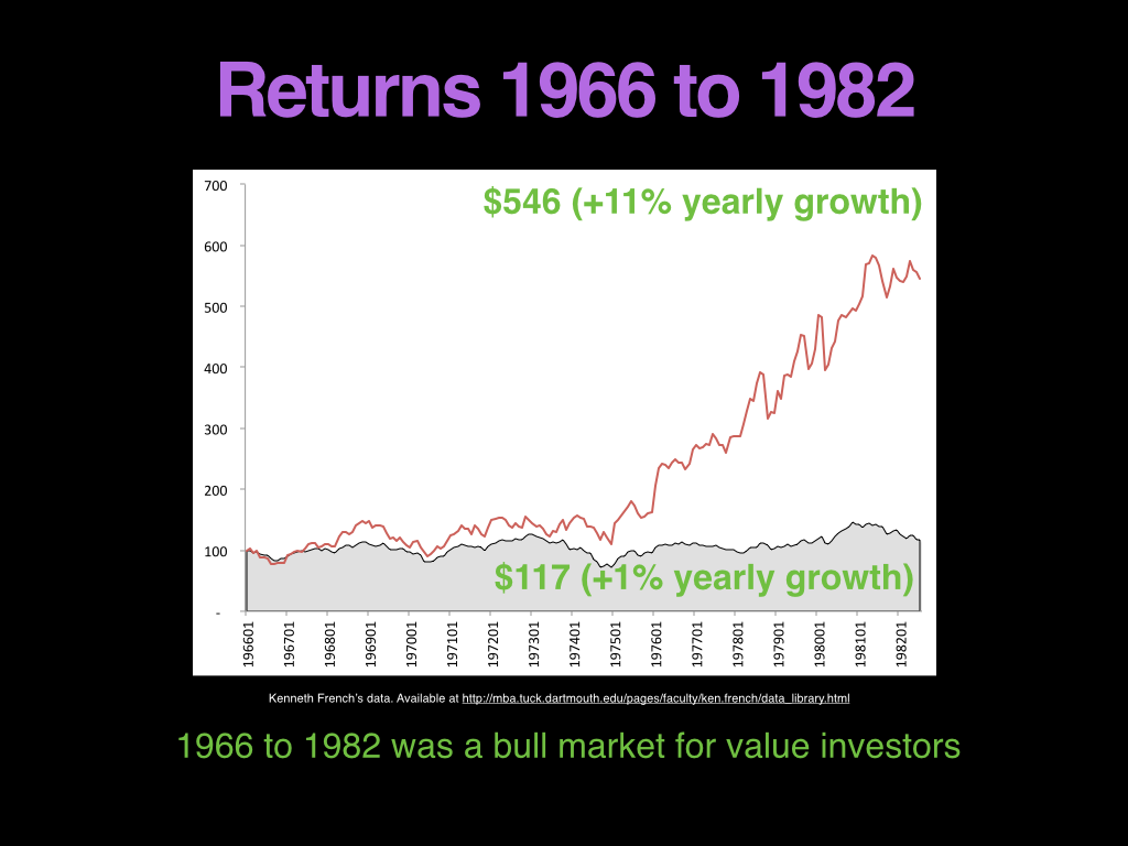
Here we use Ken French’s P/B value decile and compare the returns to the S&P500 over the same period. (It’s not an entirely fair fight because the value decile draws from smaller stocks than the S&P500, but so can we, so that’s what I’m using.)

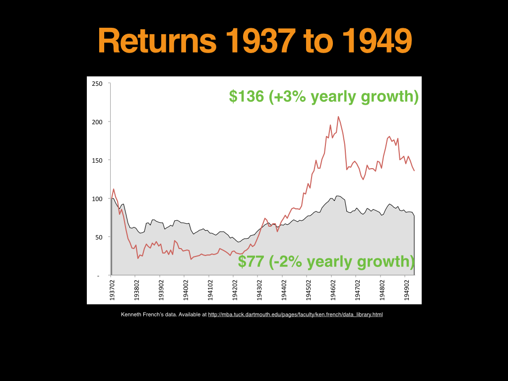
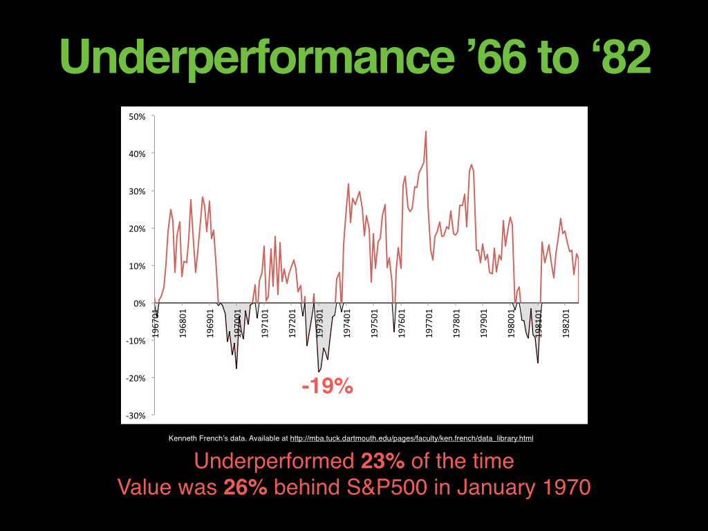
Value made its own way, but it beat out the S&P500 over the full period. The 1966 to 1982 sideways market was a genuine bull market for value investors.

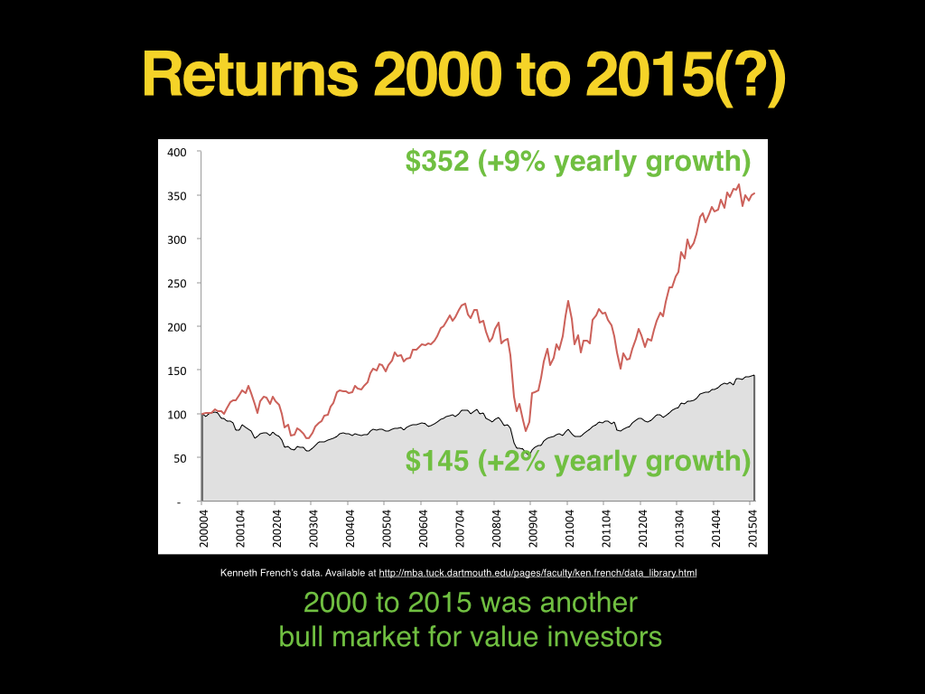
And the 2000s have been kind to value investors too.

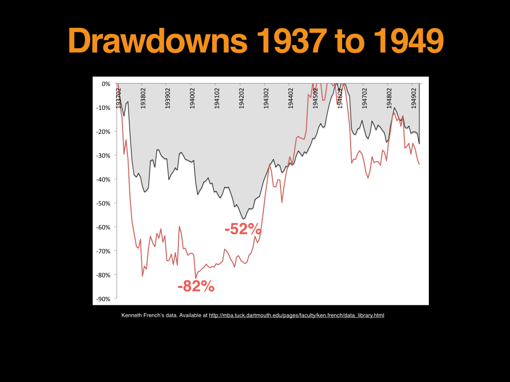
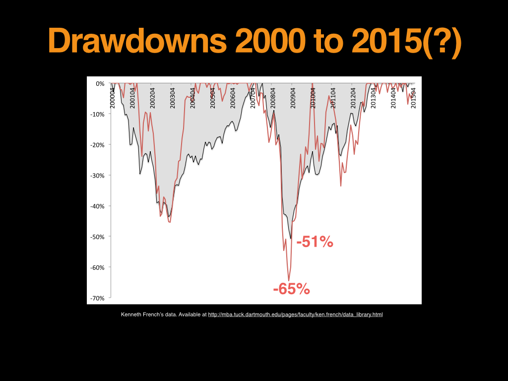
Of course, there’s nothing free in this world. The tradeoff for beating the market over the full period is big drawdowns and lots of underperformance. Look at the blockbuster drawdown for value in the early 1940s. You’d just about give the game away down 82 percent.

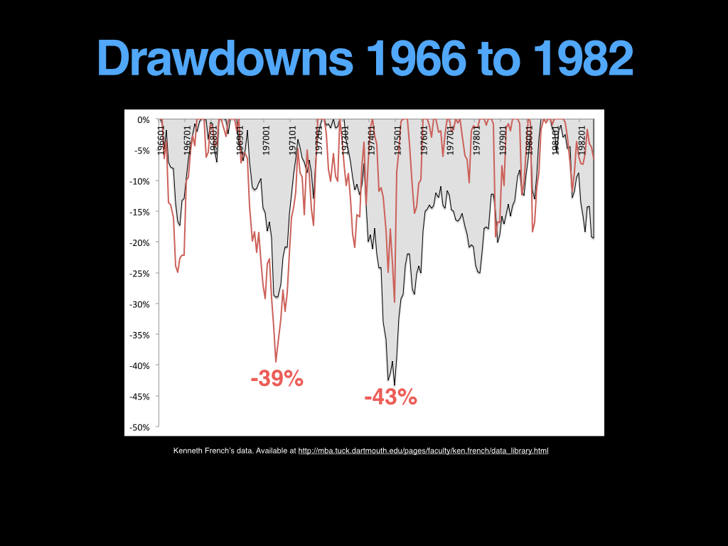
1966 was more benign, but there were lots of drawdowns on the way to those great returns.

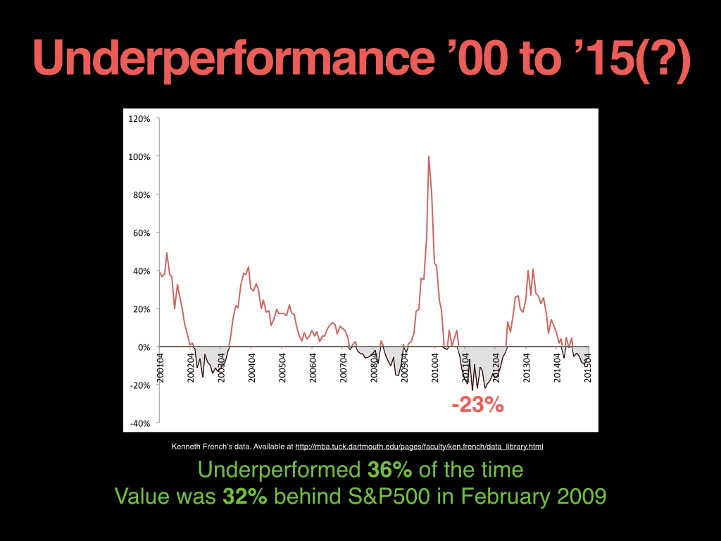
2000 on has taken some wild spills too. 2009 was tough one.

Value underperformed a lot in the 1937 to 1949 sideways market. At one stage it was 66 percent behind the market.

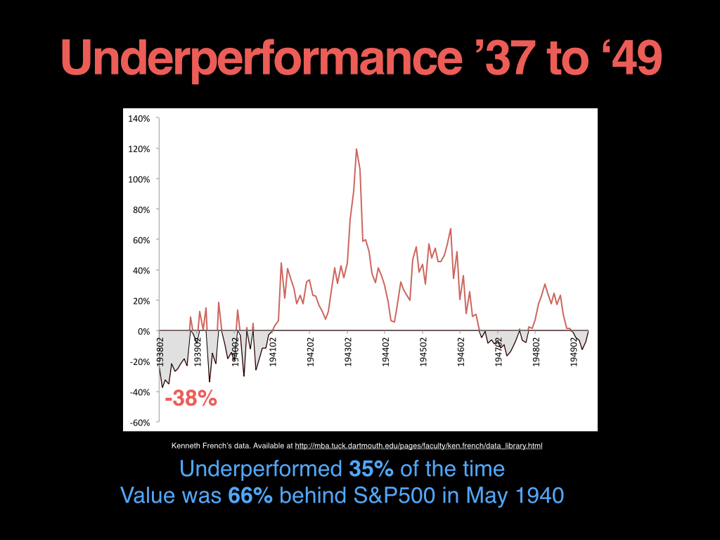
’66 was easier, but it lagged by 26 percent in the early 1970s.

And there have several periods of underperformance over the last 15 years to get the great outperformance.

If you’ve got the stomach for it, value is a great way to ride out a sideways market. (In a bull market, you just throw a dart at index and head to the beach).

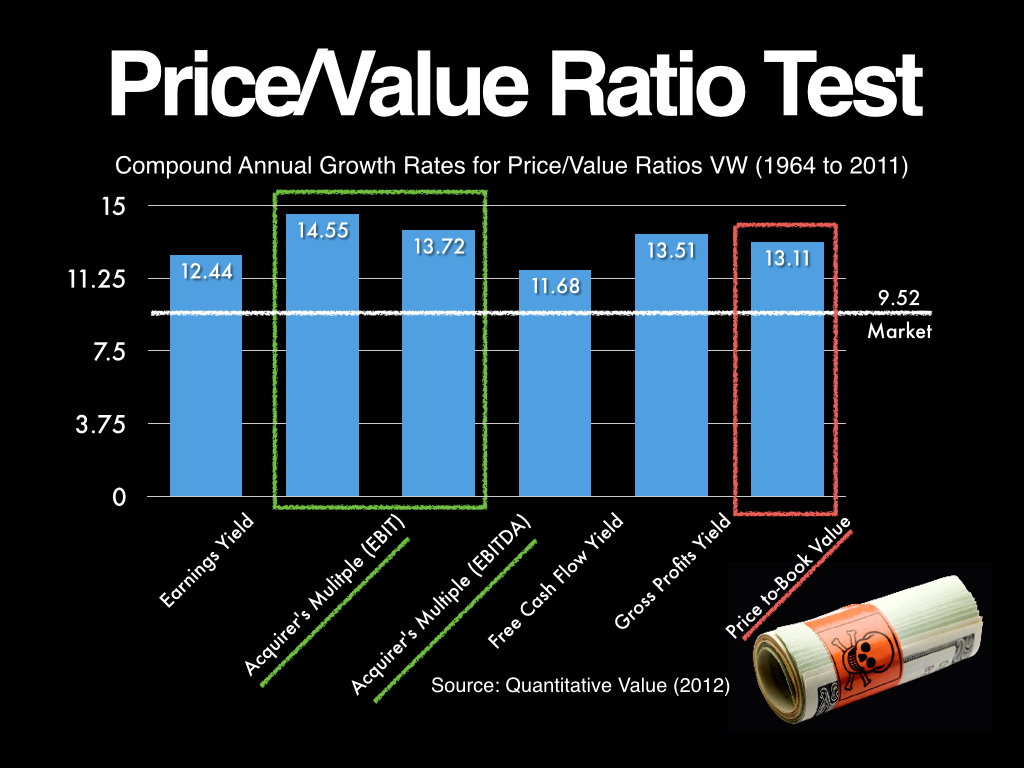
If you’re going to focus on value, the acquirer’s multiple is the way to go. It’s beaten out book value (and every other metric) in the best data we have: